采用SPSS进行Two-way ANOVA统计分析
2013-10-15 MedSci MedSci原创
Two-way ANOVA统计在临床应用中并不多,但偶然能遇到。在老版本的SPSS中容易处理,但是在最新的SPSS中,如SPSS 19.0后,找不到Two-way ANOVA选项。到底如何处理呢?有时投稿时,审稿人也会要求进行Two-way ANOVA,如:“Since treatment and time course was investigated, two way ANOVA follo
有时投稿时,审稿人也会要求进行Two-way ANOVA,如:“Since treatment and time course was investigated, two way ANOVA followed by post hoc test should be applied”.以前习惯于在SPSS中用one-way ANOVA ,那么two-way在哪呢?如何安排数据?如何统计?如何看结果?在网上搜索了很多资料,发现有一篇文章实用、详细而全面介绍了如何在SPSS使用two-way ANOVA(我的SPSS 版本是16,如下文运新two-way ANOVA 没有问题,但是在Syntax(用于比较同一treatment下不同时间之间差异或则同一时间点各treatment之间的差异)时界面不同)。
具体做法,采用广义因素分析过程,即采用广义线性模型(General Linear
Models)模块的一个子模块,用于分析多个因素(变量)对一个因素(反应变量)的影响,包含了一般的方差分析内容,如完全随机设计资料的方差分析
(one way ANOVA),随机单位组设计资料的方差分析(two-way ANOVA),拉丁方设计资料的方差分析(three-way
ANOVA),析因分析(factorial analysis),交叉设计(cross-over design),正交设计(orthogonal
design),裂区设计(split-plot
design)资料的方差分析,协方差分析,重复测量数据的方差分析等。在SPSS新版本中,Two-way
Anova分析即采用广义线性模型(General Linear Models)进行分析。具体步骤如下:
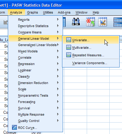
方法:使用SPSS中的Analyze----General linear model-----Univariate
(1)依次点击SPSS中的Analyze----General linear model-----Univariate
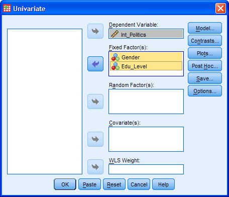
(2)把因变量(成绩)放入 DEPENDENT VARIABLE 方格中;把所有自变量放入 FIXED FACTORS方格中;
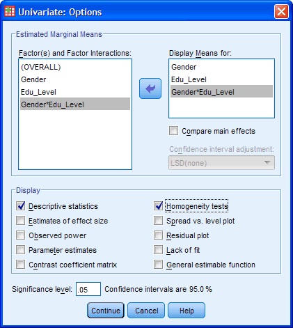
(3)点击OPTIONS,然后在ESTIMATED MARGINAL MEANS 中把所有的因素拖到DISPLAY MEANS FOR的方格中;
(4)在DISPLAY区域选中DESCRIPTIVE STATISTICS和ESTIMATES OF EFFECT SIZE boxes;然后点击Contintue回到Univariate主窗口;
(5)如何任何变量有 3个或3个以上的情况,则需要点击POST-HOCS,把超过3种情况的变量拖入POST-HOC TESTS FOR方格。
(6)在EQUAL VARIANCES ASSUMED区域里选择TUKEY;
(7)点击CONTINUE回到 UNIVARIATE主窗口并点击OK
Introduction
The two-way ANOVA compares the mean differences between groups that have been split on two independent variables (called factors). You need two independent, categorical variables and one continuous, dependent variable (see our guide on Types of Variable).
Assumptions
- Dependent variable is either interval or ratio (continuous) (see our guide on Types of Variable)
- The dependent variable is approximately normally distributed for each combination of levels of the two independent variables (see our Testing for Normality guide, which deals specifically with the two-way ANOVA).
- Homogeneity of variances of the groups formed by the different combinations of levels of the two independent variables.
- Independence of cases (this is a study design issue and is not addressed by SPSS).
Example
A researcher was interested in whether an individual's interest in politics was influenced by their level of education and their gender. They recruited a random sample of participants to their study and asked them about their interest in politics, which they scored from 0 - 100 with higher scores meaning a greater interest. The researcher then divided the participants by gender (Male/Female) and then again by level of education (School/College/University).
Setup in SPSS
In SPSS we separated the individuals into their appropriate groups by using two columns representing the two independent variables and labelled them "Gender" and "Edu_Level". For "Gender", we coded males as "1" and females as "2", and for "Edu_Level", we coded school as "1", college as "2" and university as "3". The participants interest in politics was entered under the variable name, "Int_Politics". To know how to correctly enter your data into SPSS in order to run a two-way ANOVA, please read our Entering Data in SPSS tutorial, where there is a specific example. The data setup can be seen in the diagram below (click image to see full data set). We have given our data text labels (see our Working with Variables guide).
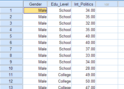
Published with written permission from SPSS Inc, an IBM Company.
Testing of Assumptions
To determine whether your dependent variable is normally distributed for each combination of the levels of the two independent variables see our Testing for Normality guide that runs through how to test for normality using SPSS using a specific two-way ANOVA example. In SPSS, homogeneity of variances is tested using Levene's Test for Equality of Variances. This is included in the main procedure for running the two-way ANOVA, so we get to evaluate whether there is homogeneity of variances at the same time as we get the results from the two-way ANOVA.
Test Procedure in SPSS
- Click Analyze > General
Linear Model > Univariate... on the
top menu as shown below:
Published with written permission from SPSS Inc, an IBM Company.
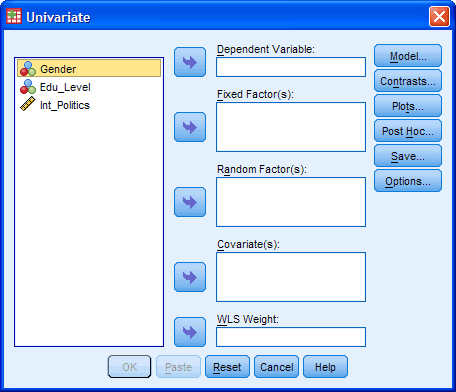
- You will be presented with the "Univariate" dialogue box:
Published with written permission from SPSS Inc, an IBM Company.
- You need to transfer the dependent variable
"Int_Politics" into the "Dependent
Variable:" box and transfer both independent variables,
"Gender" and "Edu_Level", into
the "Fixed Factor(s):" box. You can do this by
drag-and-dropping the variables into the respective boxes or by
using the
 button. If you are using older versions of SPSS you
will need to use the former method. The result is shown below:
[For this analysis you will not need to worry about the "Random Factor(s):", "Covariate(s):" or "WLS Weight:" boxes.]
Published with written permission from SPSS Inc, an IBM Company.
- Click on the
 button. You will be presented with the "Univariate:
Profile Plots" dialogue box:
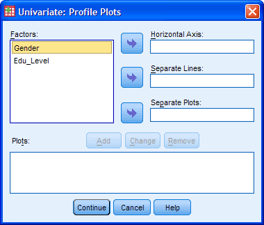
Published with written permission from SPSS Inc, an IBM Company.
- Transfer the independent variable "Edu_Level" from the "Factors:" box into the "Horizontal Axis:" box and transfer the "Gender" variable into the "Separate Lines:" box. You will be presented with the following screen:
[Tip: Put the independent variable with the greater number of levels in the "Horizontal Axis:" box.]
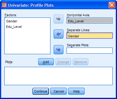
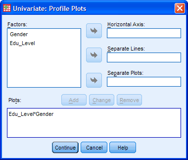
Published with written permission from SPSS Inc, an IBM Company.
You will see that "Edu_Level*Gender" has been added to the "Plots:" box.
- Click the
 button. This will return you to the "Univariate"
dialogue box.
 - Click the
 button. You will be presented with the "Univariate:
Post Hoc Multiple Comparisons for Observed..." dialogue box as
shown below:
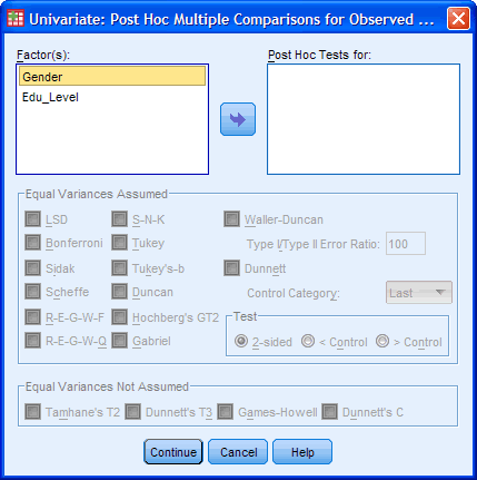
Published with written permission from SPSS Inc, an IBM Company.
Transfer "Edu_Level" from the "Factor(s):" box to the "Post Hoc Tests for:" box. This will make the "Equal Variances Assumed" section become active (loose the "grey sheen") and present you with some choices for which post-hoc test to use. For this example, we are going to select "Tukey", which is a good, all-round post-hoc test.
[You only need to transfer independent variables that have more than two levels into the "Post Hoc Tests for:" box. This is why we do not transfer "Gender".]
You will finish up with the following screen:
Click the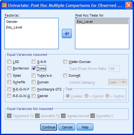
Published with written permission from SPSS Inc, an IBM Company.
 button to return to the "Univariate" dialogue
box.
- Click the
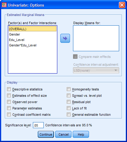
 button. This will present you with the "Univariate:
Options" dialogue box as shown below:
Published with written permission from SPSS Inc, an IBM Company.
- Transfer "Gender",
"Edu_Level" and
"Gender*Edu_Level" from the "Factor(s)
and "Factor Interactions:" box into the "Display
Means for:" box. In the "Display" section, tick the
"Descriptive Statistics" and "Homogeneity tests"
options. You will presented with the following screen:
Published with written permission from SPSS Inc, an IBM Company.
Click the
 button to return to the "Univariate" dialogue
box.
 - Click the
 button to generate the output.
SPSS Output of Two-way ANOVA
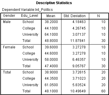
SPSS produces many tables in its output from a two-way ANOVA and we are going to start with the "Descriptives" table as shown below:
Published with written permission from SPSS Inc, an IBM Company.
This table is very useful as it provides the mean and standard deviation for the groups that have been split by both independent variables. In addition, the table also provides "Total" rows, which allows means and standard deviations for groups only split by one independent variable or none at all to be known.
Levene's Test of Equality of Error Variances
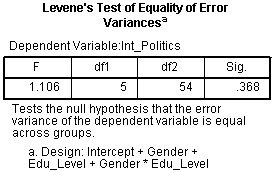
The next table to look at is Levene's Test of Equality of Error Variances as shown below:
Published with written permission from SPSS Inc, an IBM Company.
From this table we can see that we have homogeneity of variances of the dependent variable across groups. We know this as the Sig. value is greater than 0.05, which is the level we set for alpha. If the Sig. value had been less than 0.05 then we would have concluded that the variance across groups was significantly different (unequal).
Tests of Between-Subjects Effects Table
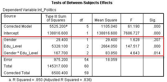
This table shows the actual results of the two-way ANOVA as shown below:
Published with written permission from SPSS Inc, an IBM Company.
We are interested in the Gender, Edu_Level and Gender*Edu_Level rows of the table as highlighted above. These rows inform us of whether we have significant mean differences between our groups for our two independent variables, Gender and Edu_Level, and for their interaction, Gender*Edu_Level. We must first look at the Gender*Edu_Level interaction as this is the most important result we are after. We can see from the Sig. column that we have a statistically significant interaction at the P = .014 level. You may wish to report the results of Gender and Edu_Level as well. We can see from the above table that there was no significant difference in interest in politics between Gender (P = .207) but there were significant differences between educational levels (P < .0005).
Multiple Comparisons Table
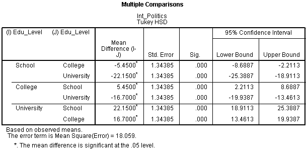
This table shows the Tukey post-hoc test results for the different levels of education as shown below:
Published with written permission from SPSS Inc, an IBM Company.
We can see form the above table that there is some repetition of the results but, regardless of which row we choose to read from, we are interested in the differences between (1) School and College, (2) School and University, and (3) College and University. From the results we can see that there is a significant difference between all three different combinations of educational level (P < .0005).
Plot of the Results
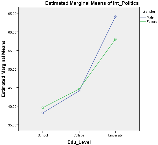
The following plot is not of sufficient quality to present in your reports but provides a good graphical illustration of your results. In addition, we can get an idea of whether there is an interaction effect by inspecting whether the lines are parallel or not.
Published with written permission from SPSS Inc, an IBM Company.
From this plot we can see how our results from the previous table might make sense. Remember that if the lines are not parallel then there is the possibility of an interaction taking place.
Procedure for Simple Main Effects in SPSS
You can follow up the results of a significant interaction effect by running tests for simple main effects - that is, the mean difference in interest in politics between genders at each education level. SPSS does not allow you to do this using the graphical interface you will be familiar with, but requires you to use syntax. We explain how to do this below:
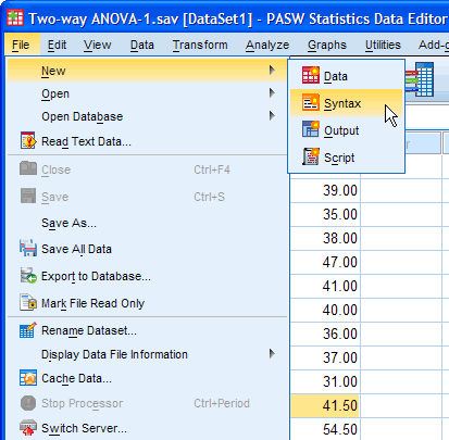
- Click File > New
> Syntax from the main menu as shown
below:
Published with written permission from SPSS Inc, an IBM Company.
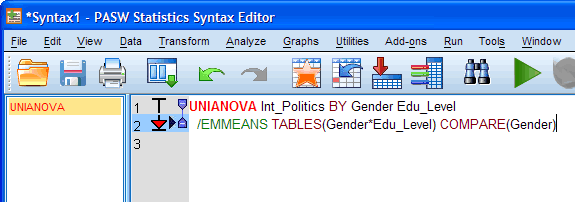
- You will be presented with the Syntax Editor as shown below:
(在SPSS 16中界面不是这样的)

Published with written permission from SPSS Inc, an IBM Company.
- Type text into the syntax editor so that you end up with the
following (the colours are automatically added):
[Depending on the version of SPSS you are using you might have suggestion boxes appear when you type in SPSS-recognised commands, such as, UNIANOVA. If you are familiar with using this type of auto-prediction then please feel free to do so, but otherwise simply ignore the pop-up suggestions and keep typing normally.](在SPSS 16中,你只管如下图右框显示输入命令,然后点击上面菜单中的Run-all,结果就输出了
 )
)
Published with written permission from SPSS Inc, an IBM Company.
Basically, all text you see above that is in CAPITALS, is required by SPSS and does not change when you enter your own data. Non-capitalised text represents your variables and will change when you use your own data. Breaking it all down, we have:
UNIANOVA Tells SPSS to use the Univariate Anova command Int_Politics BY Gender Edu_Level Your dependent variable BY your two independent variables (with a space between them) /EMMEANS Tells SPSS to calculate estimated marginal means TABLES(Gender*Edu_Level) Generate statistics for the interaction term. Put your two independent variables here, separated by a * to denote an interaction COMPARE(Gender) Tells SPSS to compare the interaction term between genders - Making sure that the cursor is at the end of row 2 in the
syntax editor click the
 button, which will run the syntax you have typed.
Your results should appear in the Output Viewer below the results
you have already generated.
SPSS Output of Simple Main Effects
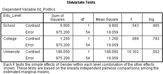
The table you are interested in is the Univariate Tests table:
Published with written permission from SPSS Inc, an IBM Company.
This table shows us whether there are statistical differences in mean political interest between gender for each educational level. We can see that there are no statistically significant mean differences between male and females' interest in politics when individuals are educated to school (P = .465) or college level (P = .793). However, when individuals are educated to University level, there are significant differences between males and females' interest in politics (P = .002).
本网站所有内容来源注明为“梅斯医学”或“MedSci原创”的文字、图片和音视频资料,版权均属于梅斯医学所有。非经授权,任何媒体、网站或个人不得转载,授权转载时须注明来源为“梅斯医学”。其它来源的文章系转载文章,或“梅斯号”自媒体发布的文章,仅系出于传递更多信息之目的,本站仅负责审核内容合规,其内容不代表本站立场,本站不负责内容的准确性和版权。如果存在侵权、或不希望被转载的媒体或个人可与我们联系,我们将立即进行删除处理。
在此留言




没有结果,不知道是因为什么原因
80
很有帮助,谢谢
182
#ANOVA#
63
感谢分享!先收了。
168